
D) Geological Models and Seismic Responses
Since current data processing and interpretation yield seismic sections resembling geologic cross-sections, inexperienced geologists and geophysics, i.e., geoscientists are, often greatly, tempted to read geology, more or less directly, from the seismic data. Serious errors may result in such approach. This is, especially, true in areas of complex tectonics (high dips), rapid changes in lithology (density and velocity), irregular surfaces and complex weathering near surface conditions.
The following geological models and their time responses indicate why so many errors are, frequently, found in tentative geological interpretations of seismic line.
When a tilting of a given sedimentary packages predates compaction, there is a natural increasing of the velocity interval with depth. In time seismic lines (by far the more used), one can say that a constant time-thickness emphasizes an increasing depth-thickness, since the velocity interval is greater in the more buried sediments.
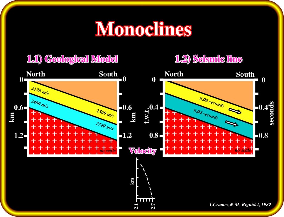
Plate 79- This sketch illustrates a monocline model and its seismic response. On seismic lines, a tilted isopach time intervals does not show, in depth sections, a constant thickness, except when the tilting of the sediments is post-compaction. In this particular example, characterized by a pre-compaction tilting (the sedimentary packages were tilted before compaction), within the same interval (yellow interval for instance), the velocity interval changes from 2130 m/s (in the area less buried) to 2560 m/s (in the area more buried). In the deepest area, the seismic waves spend less time to travel the same distance (less 0.04 sec. t.w.t.).
A mathematical geological model of a pre-compaction tilted stratigraphic column and its wave equation seismic response are illustrated above (Plate 79). The time thickness of each sedimentary package is thinning down-dip. However, in the mathematical depth model the thickness is constant, just the velocity interval increases downward.
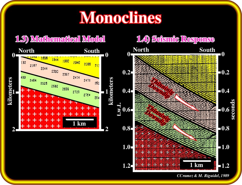
Plate 80- In the mathematical model, three isopach interval are considered. In each interval, due to differential burial the compressional wave velocity increases down-dip. In the uppermost interval (yellow), the velocity ranges from 1804 to 2136 m/s. In the second interval (rose), the velocity is higher. It ranges from 2130 m/s, in the less buried sediments, to 2520 m/s, in the more deeply buried sediments. In the green interval, overlying the basement, the velocities change from 2400 to 2840 m/s. In spite of the fact that in the model, the intervals are isopachous, they are thinning down-dip on the seismic response.
In geological terms, this mathematical model is no too natural. In fact, to get in the field, after compaction an isopach interval with a progressive increasing of the velocity interval down-dip, it means that at deposition time the interval was thicker where is now denser and that the increasing in thickness was balanced by the compaction (increasing with the burring)
D.2- Normal Faults (growth faults)
On a seismic line, the majority of the normal faults have a geometry similar to that illustrated on Plate 81, that is to say, the reflector of the up-thrown block (hanging-wall), below the fault plane, is pulled down, while on the ground, or in the geological depth model (see below) the reflectors are roughly horizontal.
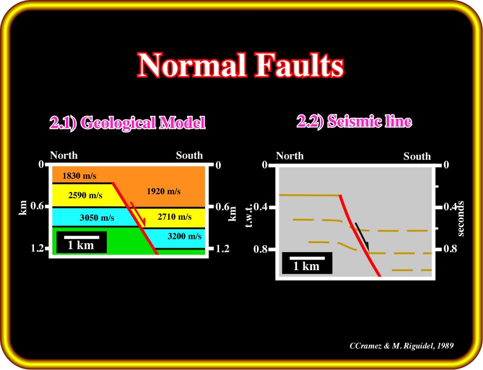
Plate 81- This plate illustrates a geological model of a normal fault (left) and its seismic response (right). Theoretically, due to the downward relative movement of the hanging-wall, intervals with quite different interval-velocities are juxtaposed, which has important consequences on the seismic response. The foot-wall reflectors, below the fault plane (area of a lateral velocity changing), will be pulled down, since, at same level, the velocity interval in the hanging-wall is smaller.
The explanation of this misleading geometry is, easily found in Plate 82. Due to the fault movement, there is juxtaposition between high velocity sediments of the up-thrown faulted block and lower velocity sediments of the down-thrown block (hanging-wall).
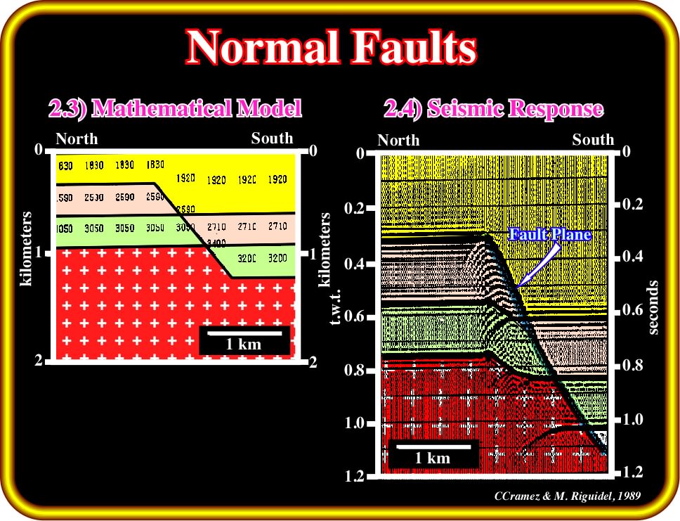
Plate 82- On the mathematical model (left), three sedimentary intervals are considered above the basement. All intervals are affected by a normal fault. The sediments of the hanging-wall (down-thrown faulted block) are denser (the fault is pre-comapction). They reached higher depths. Their compressional wave velocities are higher than the sediments of the foot-wall. On the seismic response, the reflectors of the foot-wall are pulled-down below the fault plane, where there is a lateral change of interval-velocity.
This seismic artifact, induced by lateral changes in the interval velocity, is recognized, easily, on seismic lines, as illustrated below on the auto-trace of a seismic line from Angola offshore (Plate 83). As the sediments of the down-thrown block of the fault-growth have a lower velocity (mainly shales) than the sediments of the up-thrown block (mainly carbonates), not only the reflections below the fault plane are pull-downed, but the reflection associated which the salt weld, as well.
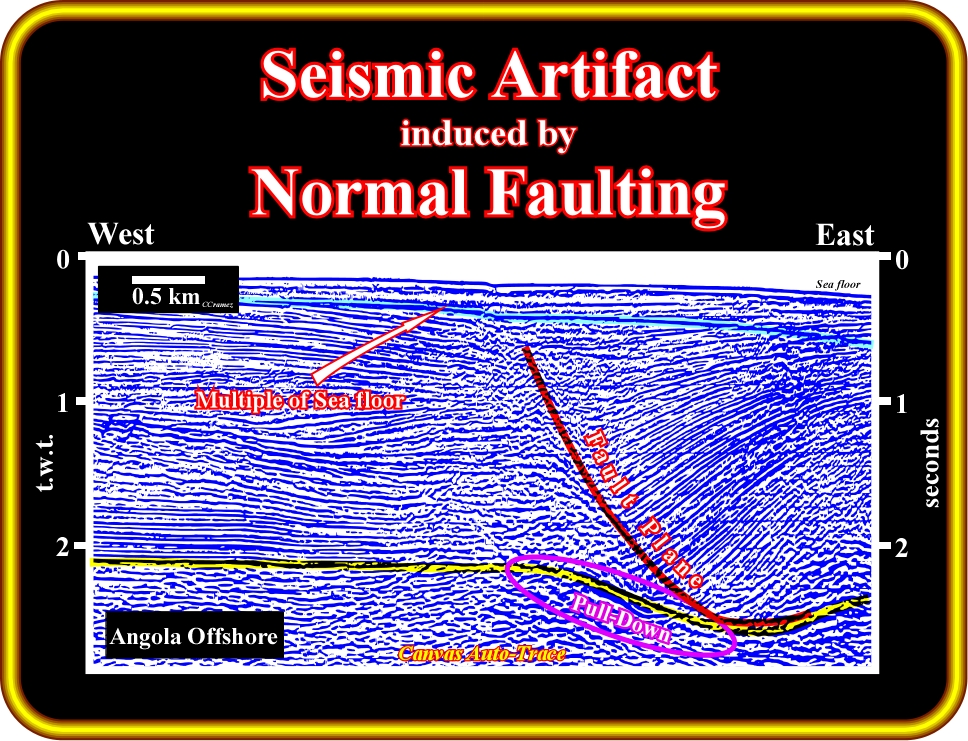
Plate 83- On this auto-trace of seismic line from Angola offshore, the pull-down of the yellow marker (bottom of the evaporitic interval) is induced by the lateral change of the interval-velocity created by the normal fault which limits a Upper Tertiary depocenter. Such a fault puts limestones (up-thrown block) and shales (down-thrown block) in juxtaposition. On a depth version of the seismic line, the tectonic disharmony induced by salt tectonics (emphasized by the yellow marker) should be, more or less, subhorizontal. Such a conjecture can be used to tentatively correct (locally) the velocity interval used in the depth conversion.
D.3- Reverse Faults (thrust faults)
On the reverse fault geological model used below, the geometry of the different sedimentary facies (lithologies) is parallel and horizontal. Interval velocities are, laterally, constant. Due to the fault movement, created by a compressional tectonic regime (sedimentary shortening), the up-thrown faulted block was uplift. Sedimentary packages with different velocity intervals are juxtaposed (lateral velocity change).
The principal consequence of such a lateral and abrupt changing of the velocity interval is the pull-up of the seismic reflectors below the fault plane, i.e., of the foot-wall. Plate 84 illustrates the velocity model used to find the more likely seismic response (time) of the previous model.
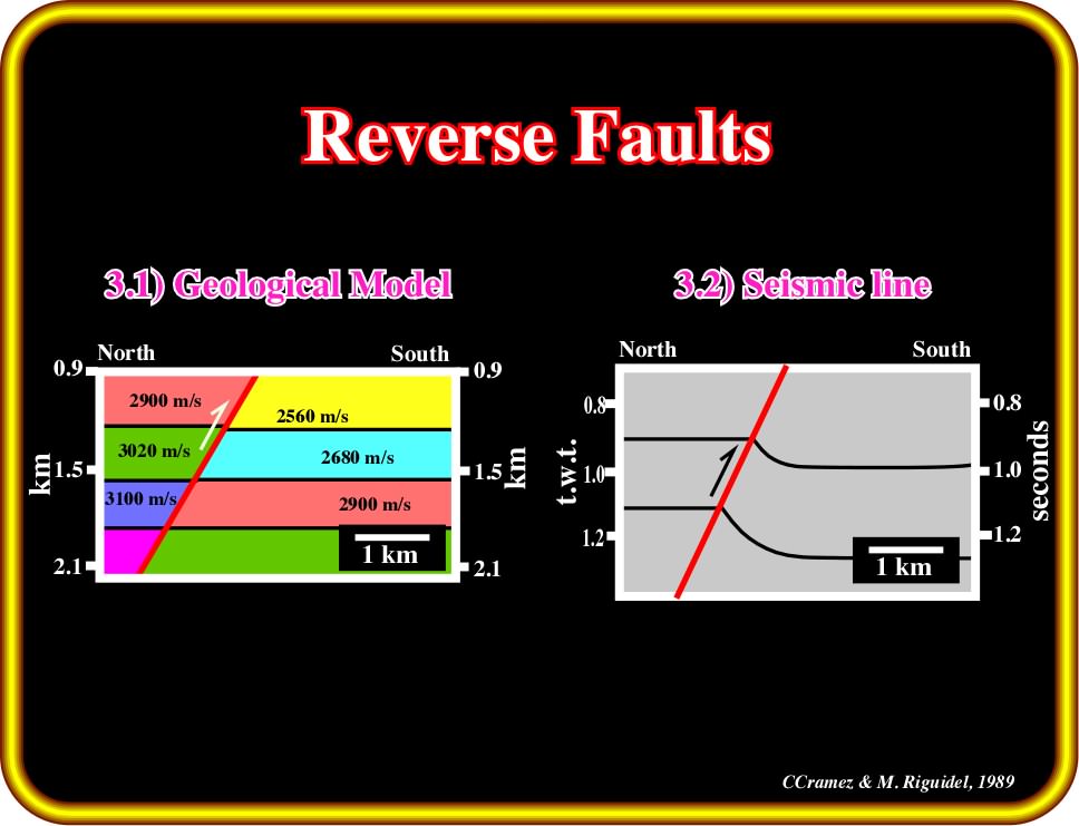
Plate 84- The geological model of a reverse fault and its likely seismic response here illustrated are quite obvious. Due to the shortening of the sediments induced by a compressional tectonic regime, the sedimentary packages of the up-thrown faulted block were uplifted. Such a discontinuous uplift put in juxtaposition sedimentary intervals with different lithologies and different compaction, since the model assumes a post-compaction faulting. There a sharp change in the velocities interval compaction between the faulted blocks. As the reverse fault is a low angle fault, on a seismic line, as illustrated on the right sketch, the reflectors of the foot-wall are pulled-up due to a lateral change of the interval-velocities.
It is, particularly, important to notice that on a seismic line, the trace of the reverse fault plane is not emphasized by an obvious reflection, but marked by the discontinuities between straight dipping reflector (on the right) and the pulled-up reflectors on the left (hanging-wall). Interpreters should not interpret the pull-up of the reflectors as a geological uplift associated with a compressional tectonic regime (as in antiform trap, for instance).
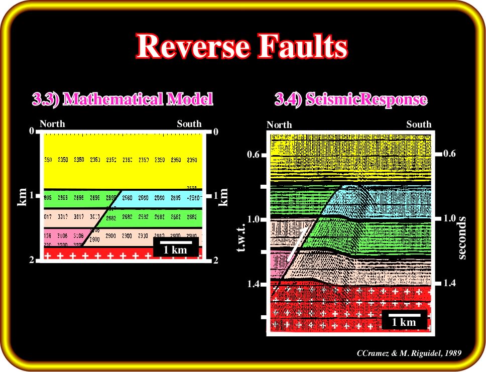
Plate 85- This seismic response (right) of a mathematical model of a reverse fault (left), in which the sediments of the hanging-wall (up-thrown block) are denser than those of the foot-wall, corroborates the hypothesis that reflectors below the fault plane are pulled-up creating the common illusion of an anticline structure (see Plate 86).
If you have doubts, to decide between a pull-up and a structural tectonic feature, do not forget that a depth conversion can solve the problem :
(i) If the antiform like feature disappears on the depth-converted section that means that it was a pull-up induced by a lateral velocity change ;
(ii) If, on the contrary, the antiform like structure persists on a depth converted line, it may be, tentatively, interpreted as sedimentary shortening in the foot-wall.
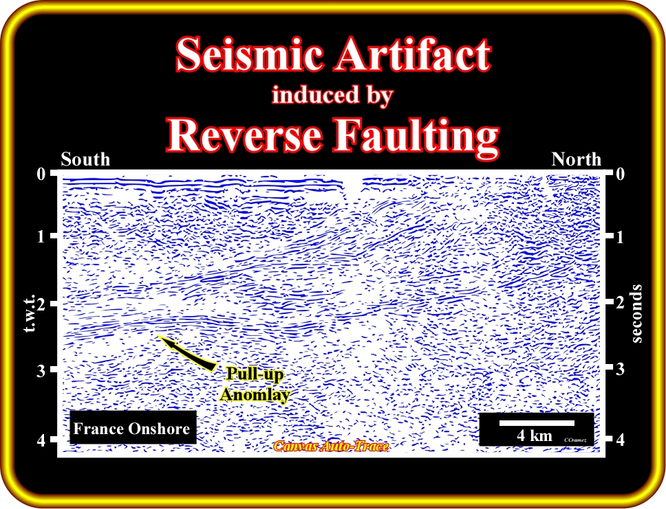
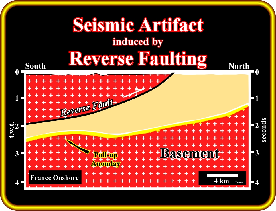
Plate 86- This tentative interpretation of an auto-trace seismic line from France onshore illustrates the seismic artifact associated with a thrust fault, i.e., an apparent anticline structure under the reverse fault plane. In spite of the evidence of the seismic pull-up, geoscientists drilled a well on such an artifact thinking that they were testing a large under-thrust structural trap. In certain basins, as we will see later, there are prolific petroleum traps under reverse and thrust faults. Geoscientists must always test their interpretations by time-depth conversions before drilling.
If you recognize an antiform feature in the foot-wall faulted block of a reverse fault you must admit two possibilities : (i) Seismic artifact ; (ii) Anticline. Then, you must, imperatively, test both hypotheses and reject the one which is more falsified by testing. In petroleum exploration, avoiding such scientific tests can be highly dangerous and expensive. PHT (Problem - Hypothesis - Test) is, by far, the best exploration method.
An example of such an exploration approach is the discovery of giant Cuisana field (Colombia). The Cusiana prospect, located on the foot-wall block of a very important reverse fault, the Yopal fault, was proposed by Triton, who held 100% of the exploration rights, to several major oil companies. The majority of the companies interpreted the structure as a pull-up due to a lateral velocity change induced by the Yopal fault, and refused Triton‘s farm-out.
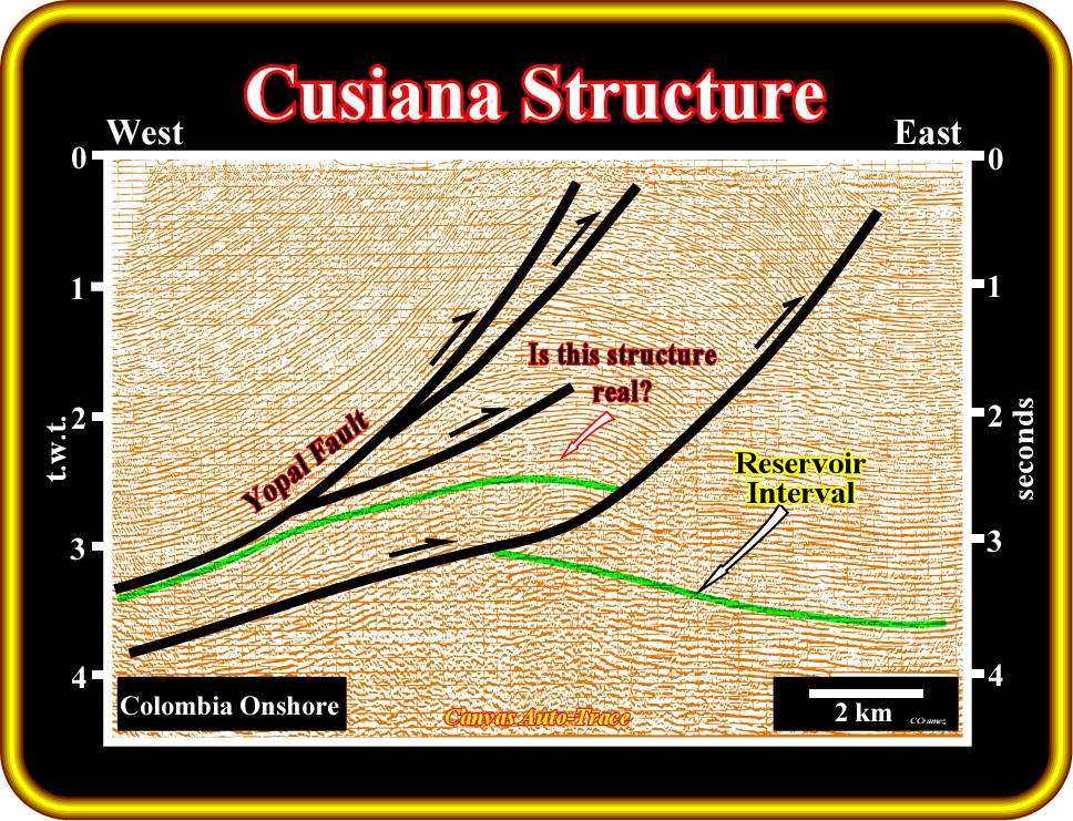
Plate 87- This auto-trace of a seismic line through Cuisiana #2A (discovery well), in the Colombia foothills, was drilled by an international consortium composed of BP, Total and Triton, in order to test the anticline structure under upper thrust-faults. Before drilling, several time-depth conversions corroborated the hypothesis advanced by certain geoscientists that the sub-thrust antiform was a real compressional structure and not a seismic artifact induced by the hanging-wall.
The tentative interpretation illustrated on Plate 87 (Cusiana prospect) was tested by several depth conversions using different velocity intervals, in order to refute the hypothesis assuming an anticline structure below the Yopal thrust fault (petroleum exploration progresses by refutation and by verification). In spite of all refutation tentatives, the presence of a significant structural trap under the Yopal thrust was, by far, the hypothesis more likely. Finally, the consortium BP, Total, Triton decide to drilled (probably more than 5 Gb of recoverable reserves).
Oil reserves comprise that oil which has been discovered and which remains unused. All discoveries are, initially, appraised for their size in terms of oil in place. Based on probabilistic estimates derived from a large number of parameters there will, subsequently be an initial declaration of recoverable oil which geological and engineering information indicates can, with reasonable certainty, be recovered in the future under existing economic and operating conditions. These constitute the so-called proven reserves of the field at that particular time. All fields will also be declared as having additional volumes of 'probable' and 'possible' reserves - with over 50% and under 50% probability, respectively, of being recoverable - from the estimated total volumes of oil-in-place in the reservoir.
Notwithstanding the discovery of Cusiana field, the majority of the proposed structural traps below the thrust fault in Colombia foot-will correspond do seismic artifacts. On this subject, Plate 88 illustrates how seismic artifacts can be tested by a time depth-conversion.
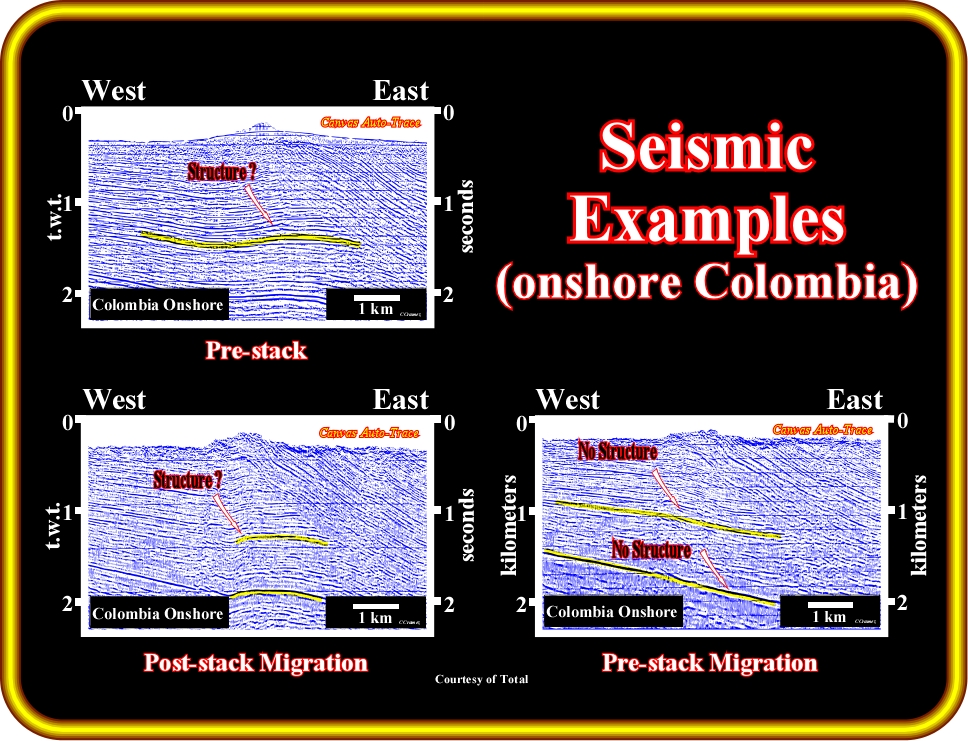
Plate 88- Not all time-depth conversions corroborate anticline structures below the thrust faults. In this particular auto-trace of seismic line coming, as the previous line, from the Colombia foothills, a nice antiform structure (that is to say a potential structural trap) is recognized on the pre-stack section. The same potential structure is, also, recognized on the pre-stack migrated version, just under the fault plane, which should make the interpretation questionable. Finally, the pre-stack migrated depth versions strongly, falsify the hypothesis of a sub-thrust structure. Actually, the sub-thrust sediments are undeformed and not shortened. ,
The example illustrated in previous plate, clearly, illustrate the danger for explorationists to make strategic decisions without testing all proposed geological hypothesis. Before selling your interpretation to the boss try to prove yourself that your interpretation is wrong, i.e., test it.
to continue press

Send E-mail to carloscramez@gmail.com or carlos.crame@bluewin.ch with questions or comments about these notes (Seismic-Sequential Stratigraphy).
Copyright © 2003 CCramez
Last modification: April, 2015
