Part I- Basic Principles in Salt Tectonics
Contents :
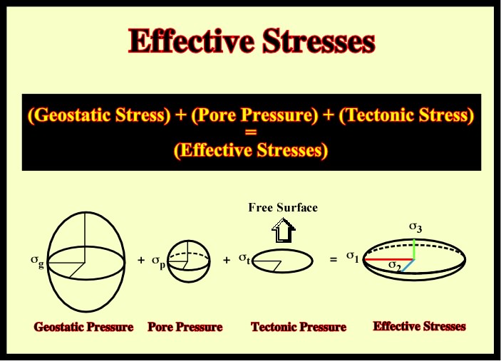
1.1- Effective Stresses
1.2- Tectonic Regimes in Sedimentary Basins
1.3- Stress Evolution in Tectonics
1.4- Salt Tectonics in Sedimentary Basins
1.4.1- Fold-Thrusts σt> 0
1.4.2- Compressive Strike-Slip, σt > 0
1.4.3- Lessening, σt > 0
1.4.4- Equilibrium (Halokinesis), σt = 0
1.4.5- Rifts - Extensional strike-slip, σt < 0
b) Growth-Faults
1.5- Summary of Salt Extensional Tectonic Deformations
1.1- Effective Stresses
What deform the sediments?
This simple question is often used to emphasize the understanding of sedimentary deformation requires the knowledge of basic principles in tectonics. In facto, the more common and erroneous answer to this is question is - the tectonic stress (σt).
The tectonic stress (σt), which can be compressive or extensive, is an un-stabilising geological factor induced by an interaction of the lithospheric plates. It, usually, acts more or less horizontally and is complementary to the lithostatic and hydrostatic pressures. When a tectonic stress (σt) is added in one direction it produces, by reaction, a lateral confining pressure (σc).
In reality, the stresses, i.e., the quantity that describes the magnitude of forces responsible for any deformation are the effective stresses (σ1, σ2, σ3), which correspond to the principal axes of the effective stresses ellipsoid (fig. 6). In a solid, stress is the force per unit area, acting on any surface within it, and variously expressed as pound or tons per square inch, or dynes or kilograms per square centimetre. By extension, the external pressure creates the interval force.
The stress at any point is mathematically defined by nine values: three to specify the normal components and six to specify the shear components, relative to three mutually perpendicular reference axes. Stress is a second rank tensor* . The forces area thought to act on every one of the infinitesimal elements of area with different orientation, which can be imagined at one point. Only such forces are considered which are, locally, in equilibrium with equal and opposite forces: tensor is symmetrical.
*Tensors are simply mathematical objects that can be used to describe physical properties, just like scalars and vectors. They are merely a generalisation of scalars and vectors; a scalar is a zero rank tensor, and a vector is a first rank tensor. The order (or rank) of a tensor is defined by the number of directions required to describe it. Properties that require one direction (first order) can be fully described by a 3×1 column vector ; properties that require two directions (second order tensors), can be described by 9 numbers, as a 3×3 matrix (generally an nth order tensor can be described by 3n coefficients.
Fig. 5- The effective stresses responsible for the deformation of the rocks are the main axes of the effective stresses ellipsoid, which is the result of the addition of the geostatic or lithostatic pressure (σg), the pore or hydrostatic pressure (p) and the tectonic stress. The geostatic pressure, at a given depth, is the vertical pressure due to the weight of a column of rock and the fluids contained in the rock above that depth (the lithostatic pressure is, often, considered, just as the vertical pressure due to the weight of the rock only. The pore pressure is the pressure of the fluid in the pore space of the rock. The tectonic stress, which is mostly horizontal, is originated from forces causing “ridge push” processes, where lithospheric plates are pushed away from a middle oceanic ridge. i.e. is the stress created by the displacement of lithospheric plates. Tectonic stress is a vector, i.e., a quantity that has both magnitude and direction, acting parallel to the surface of the geoid (shape that the ocean surface would take under the influence of the gravity of Earth, including gravitational attraction ans Earth's rotation, if other influences such as winds and tides were absent, HTTPS://wikipedia. or/wiki/Geoid).
At a given depth, the geostatic (σh), considered in these notes as equivalent to the lithostatic stress, is the stress caused by the weight of a column of the overlying beds and and the fluids contained in the rock above that depth. It can be represented by a biaxial ellipsoid: σvertical (σv = d . g . h), and horizontal (σh= confining pressure of σh).The geostatic stress ellipsoid varies with depth. The state of stress tends to become hydrostatic at great depth.
At a given depth, the pore pressure or hydrostatic stress (p) is the pressure of the interstitial fluids. It can be pictured by a uniaxial ellipsoid, which radius is ^: pore (p = d’. g . h.). In geology, the fluid, generally water, saturating the open pore spaces of a rock column, has the same effect as immersing a rock in a water column.
Using effective stresses (σ, σ2, σ3
A geologist recognizing on a time contour map several cylindrical anticline and syncline structures striking North-South, using the table I, he can put forward a compressional tectonic regime, characterised by an effective stresses ellipsoid with σ12horizontal striking N-S and σ3 2In addition, if normal-faults are pictured on the time contour map, he can say they pre-date or post-date the tectonic regime (cannot be contemporaneous of the deformation). He can say the normal-faults are, likely, posterior to the deformation otherwise they should be reactivated as reverse-faults. A reactivated normal fault can keep their original normal geometry, on the lower section of the fault plane (beneath the « null point »), when the amplitude of the inversion is not big enough.
Finally, he can hypothesize whether the basement is involved or not. In the first hypothesis, generally, tectonic disharmonies are absent. There is a roughly concordance between the deformation of basement and the cover. In the second hypothesis, generally, there is one or several mobile layer (shale or salt) within the cover creating sharp tectonic disharmonies. The overburden and the infra-mobile layer strata show, completely, different deformations.
In Table I, “Salt Tectonics” and “Halokinesis”, which are the main subjects of these notes, are depicted on the two last rows of the rock’s deformations, in which, the basement is not involved and the mobile layer is mainly composed by evaporites.
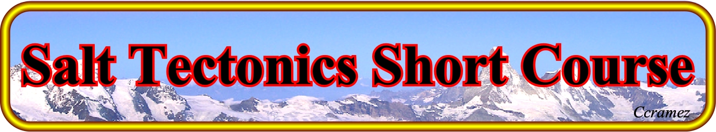
1.2- Tectonic Regimes in Sedimentary Basins
Table I
In this classification of the tectonic regimes, it is important to notice that with a positive σt the sediments can be lengthened. In other words, the term compression does not imply, necessary a positive σt. Compression means shortening of the sediments, which can be done either by folding or reverse faulting, while extension means lengthening, which can just be done by normal faulting. The strike of the fault planes (normal or reverse) is always parallel to the middle effective stress, that is to say, to σ2.
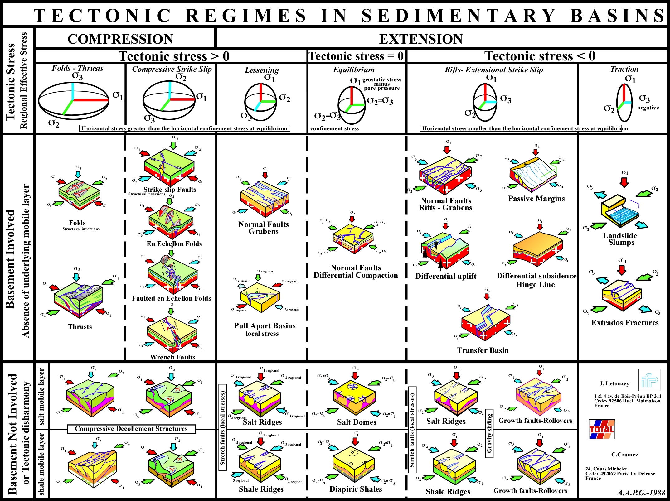
1.3- Stress Evolution in Tectonics
Depending on the geostatic (σg) and tectonic stress (σt), the effective stresses ellipsoid changes in time and space (fig. 6). When the tectonic stress (σt) is positive (right side of fig. 6), the effective stresses ellipsoid can be vertically oblong or horizontal. Conventionally, when σ1 is vertical, the sediments are lengthened (extension) by normal-faults striking parallel to the σ2. Contrariwise, when σ1 is horizontal, the sediments will be shortened whether by folding or reverse faulting. In this last hypothesis, if σ3 is vertical, the sediments will be shortened by conical-folds (en échellon-folds) and thrust faults, if σ2 is vertical the sediments will be shortened by by compressional strike slip-faults when.
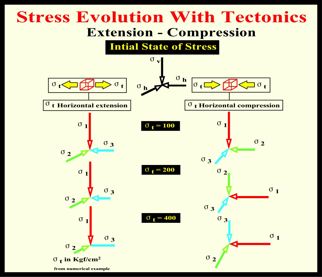
Fig. 6- This sketch summarize all possible ellipsoids of effective stresses (σ1, σ2, σ3) when a negative (extension) and a positive (compression) tectonic stress (σt) were added (100, 200 and 400 kgf/cm2) at an initial state of stress (σv , σh). At a given depth point, the state of stress corresponds to the addition of σg and σp. One can say the state of stress corresponds to the σg decreased of the σp. Hydrostatic pressure acts in opposite sense of geostatic pressure. The left column pictures the extensional tectonic regimes, in which σ1is vertical and by which the sediments will be lengthened. The right column pictures the tectonic regimes induced by a σt> 0. When σt is too small (100 kgf/cm2), sediments will be lengthened (extension). When σt is big enough to balance the geostatic pressure, sediments will be shortened whether by cylindrical-folds and reverse-faults (σ3 vertical) or by conical-folds and compressional strike slip-faults (σ2 vertical).
To understand the stress evolution with tectonics (fig.6) let’s assume : (i) homogeneous and continuous rocks (viscous-elastic behaviour) with an undeformed planar surface, at a middle depth and (ii) the confining pressure is, roughly, 8/10 of the geostatic pressure (σh = 8/10 σg).
At a given point 3000 meters depth, with an average sedimentary density of 2.5 g/cm3 and with an interstitial fluid density of 1.1 g/cm3 (water), the geostatic pressure, which is given by a biaxial ellipsoid, with σvertical = 750 kg/cm2 and σhorizontal = 8/10 of σvertical = 8/10 (750) = 600 kg/cm2. The hydrostatic pressure is given by a uniaxial ellipsoid, with σvertical = 3000 m x 1,1 g/cm3 x 9,8 m /s = 330 kg /cm2. The effective vertical pressure is given by the geostatic pressure minus the hydrostatic pressure. It corresponds to a biaxial ellipsoid, with σvertical = 750 - 330 = 420 kg/cm2 and σhorizontal= 600 - 330 = 270 kg/cm2.
Knowing the effective vertical pressure one can now add a negative or positive tectonic stress (σt = n kg/cm2) along the direction of the horizontal axis Y with an associated lateral stress (confining pressure), along the perpendicular axis (X), assumed to be half (5/10) of the amount of the tectonic stress.
Adding a negative or extensive tectonic stress along the axis Y:
Adding a tectonic stress of -100 kg /cm2 along the axis Y, we get a tridimensional ellipsoid with : σ1 = 420 kg/cm^2 ; σ3 = 270 - 100 = 170 kg/cm2 ; σ2= 270 - 5/10 (100) = 220 kg/cm2.
Adding a tectonic stress of - 200kg /cm2 along the axis Y, we get a tridimensional ellipsoid with :σ1 = 420 kg/cm2 ; σ3 = 270 - 200 = 70 kg/cm2 and σ2 = 270 - 5/10 (200) = 170 kg/cm2.
Adding a tectonic stress of - 400kg/cm2 along the axis Y, we get a tridimensional ellipsoid with : σ1 = 420 kg/cm2 ; σ3 = 270 - 400 = -130 kg/cm2 ; σ2 = 270 - 5/10 (400) = 200 kg/cm2.
Adding a positive or compressive tectonic stresses along the same axis (Y):
Adding a tectonic stress of 100kg /cm2 along the axis Y, we get a tridimensional ellipsoid with: σ1 = 420 kg/cm2 ; σ1 = 270 + 100 = 370 kg/cm2 ; σ3 = 270 + 5/10 (100) = 320 kg/cm2.
Adding a tectonic stress of 200kg /cm2 along the axis Y, we get a tridimensional ellipsoid with: σ2 = 420 kg/cm2 ; σ1 = 270 + 200 = 470 kg/cm2 ; σ3 = 270 + 5/10 (200) = 370 kg/cm2.
Adding a tectonic stress of 400kg /cm2 along the axis Y, we get a tridimensional ellipsoid with : σ2 = 420 kg/cm2 ; σ1 = 270 + 400 = 670 kg/cm2 ; σ3 = 270 + 5/10 (400) = 470 kg/cm2.
As said previously, when σ1 is vertical, sediments are lengthened by normal faults striking parallel to the σ2. The amplitude of the tectonics stress (σt) does not change the orientation of the principal axes of the effective stresses ellipsoid (σ1, σ2, σ3). Just the throw of the normal-faults becomes, progressively, higher as the tectonic stress increases.
1.4- Salt Tectonics in Sedimentary Basins
Table II
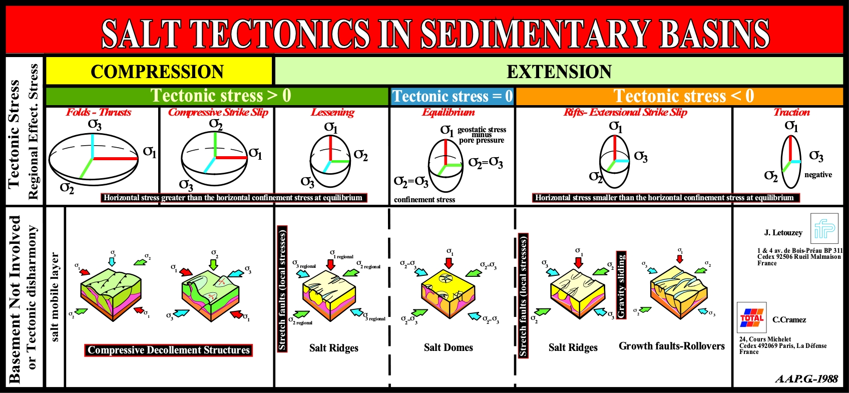
This table is a detail of Table I and summarizes the main salt structures induced by the different tectonic regimes. When the mobile layer is mainly composed by evaporites and particularly by salt, the equilibrium state, characterized by an ellipsoid of the effective stress with σ1 vertical and σ2 and σ3 equal and horizontal, is known as halokinesis.
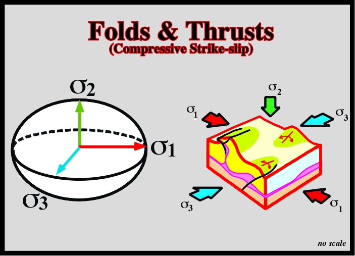
1.4.1- Folds & Thrusts, σ3 > 0 (see Table II)
Under a tectonic regime characterized by an effective stresses ellipsoid with σ1 horizontal and σ3. Depending of the rheology and geometric configuration of the sediments, a stress field can affect an area without apparent deformation. In a compressional tectonic regime, deformations are, often, confined to deformation tracks or "couloirs". Rigid blocks transmit stresses without apparent deformations.
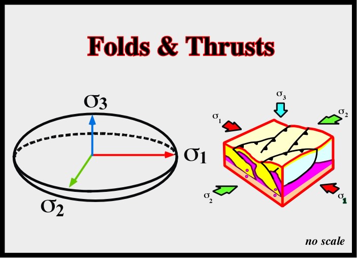
Fig. 7- A compressional σ3 tectonic regime with a σ3 vertical shortens the sediments by cylindrical folding and reverse faulting. The sediments are shortened and uplifted, since σ3 is vertical. The axes of the folds are perpendicular to σ1 and the associated faults (reverse and thrust) strike more or less parallel to σ2, following the Mohr’s circle failure principle. The inter-bedded salt layer is deformed in concordance with the overburden. However, later, , the salt layer can be deformed, locally by halokinesis, whenever the effective stresses ellipsoid becomes vertically oblong and biaxial (σ1 vertical, σ2 = σ3).
As σ3 is vertical, the sediments may be lifted above regional datum. This uplift creates a relative sea-level fall, which induces an erosional surface, that is to say, an unconformity, which may be fossilized by onlapping of recent sediments. The salt layer is deformed in concordance with the overburden. Halokinesis can pre-date or post-date the compressional deformation, depending on the geological history of the considered basin (halokinesis will be studied later). On the ground, as well as, on geological and geophysical maps, cylindrical-folds strike roughly parallel the medium effective stress, σ2. Reverse-faults and thrust-faults strike also parallel to σ2
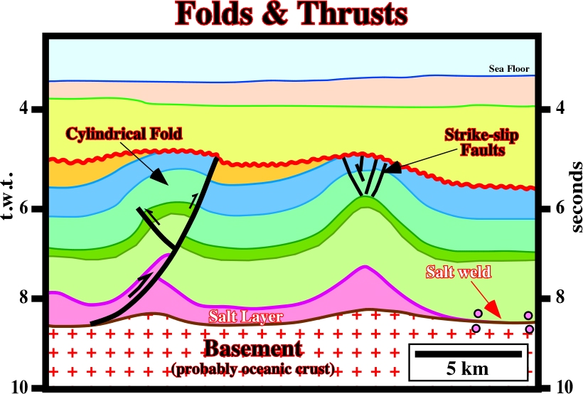
Fig. 8- On this example, the sediments below the red unconformity were shortened by a compressional tectonic regime. Halokinesis seems restricted to right end of the line, where a salt weld (see later) is well marked. The cover (salt + overburden below the red unconformity) is pre-kinematic. There are not syn-kinematic layers as usually in the halokinesis. The faults in the apex of the salt anticline, located at the right, are compressional strike-slip faults and not normal faults. They are contemporaneous of deformation. The faults on the left structure (cylindrical fold) are contemporaneous of the deformation. They are reverse-faults.
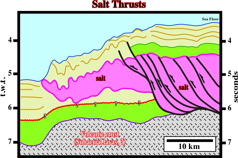
Fig. 9- Salt thrust-faults are quite frequent in the deep offshore, near the seaward limit of salt deposition, where salt interval is, often, thickened by thrusting. In this particularly example (Angola offshore), they were created by local compressional tectonic regimes induced by coeval up-dip extension along the continental slope. Sometimes, they are associated with allochthonous salt as it is the case here. Notice, that a simple depth conversion shows a huge landward step, on the top of the volcanic crust (probably sub-aerial volcanism, i.e., lava-flows), which can be interpreted as the seaward western limit of the salt deposition.
1.4.2- Compressive Strike-Slip, σ3> 0 (see Table II)
This tectonic regime is frequent in sedimentary basins associated with the formation of mega-sutures, particularly in episutural and perisutural basins. In such geological contexts, the basement is, generally, involved in the deformation and evaporitic deposits are not too frequent. However, the Neunquen geographic basin (fig. 11), in South America, and the Salt Ranges, in Pakistan, are meaningful exceptions.
When thick evaporite intervals are frequent, as in the case in South Atlantic margins, either Angola or Brazil offshores, this compressional tectonic regime, which is characterized by σ2 vertical, is often found in association with fracture zones. In fact, it is well known that (i) changes in the rate of sea floor spreading, (ii) lithospheric plates readjustment or (iii) ridge-push forces, can reactivate the fracture zones creating compressional structures in the cover. Generally, the more common structures are conical anticlines with the salt in the core of the structure (in contrast to a cylindrical anticline, a conical anticline when pictured in a stereographic projection lies in a parallel and not in a meridian). However, when the amplitude of the lateral displacement is quite significant (> 5 km), folding cannot accommodate the shortening of the cover, thereby faulting takes also place. In North Sea, this tectonic regime is found in association with the reactivation of old normal faults (tectonic inversion), particularly when the σ1
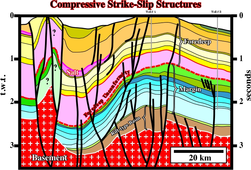
Fig. 11- This seismic line, from the Neuquen basin (onshore Argentine), illustrates a compressive strike-slip shortening of the fore-deep sediments, in which a Cretaceous evaporitic layer (Hutrim formation) was deformed in concordance with all other intervals. Similarly, but no so evident, an Oxfordian salt layer (Auquilco formation) was inverted (inverted rift-type basin in lower middle part of the line) with development of “en echelon folds” in the up-thrown faulted block. Notice, that two different compressional tectonic regimes, one with the basement involved and a younger without involvement of the basement can also explained the deformation recognized on this line.
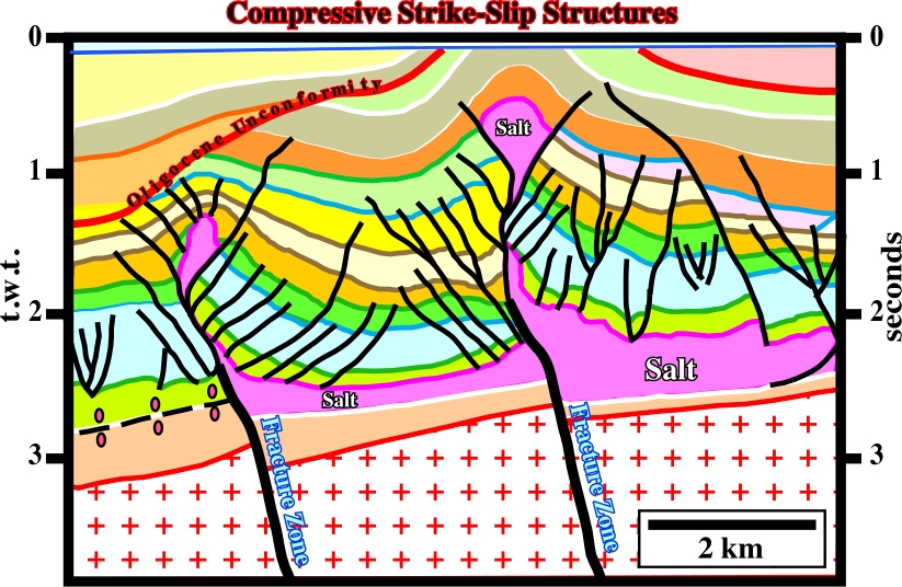
Fig. 12- Compressive strike-slip structures (faulted conical-folds) induced by reactivation of fracture zones are frequent in South Atlantic margins. Loeme salt (Kwanza and South Congo basins) forms often the core of anticline structures. Similarly, the Oligocene unconformity is uplifted and locally eroded before being fossilised by Tertiary deep-water deposits. Notice than the reactivation of the fracture zones displaces the bottom of the salt. Their movement has a compressional component. However, a later phase of halokinesis strongly deformed (uplifted) the sediments as well as the Oligocene unconformity.
1.4.3- Lessening, σ1 > 0 (see Table II)
As depicted on Table I and II, this tectonic regime is characterized by an effective stresses ellipsoid with σ1> 0, but not big enough to invert the biaxial vertically oblong state of stress ellipsoid. Generally, it is found on the distal part of foredeep basins, far away from the folded belt. As illustrated in fig. 14, the tectonic stress decreases with the distance to the frontal-thrusts of the folded-belt.
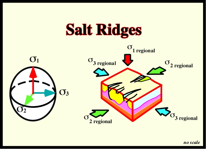
Fig. 13- When an evaporitic interval is present in a stratigraphic column undergone a tectonic regime with σ1 vertical created by a σt> 0, it is deformed into more or less parallel salt ridges. In fact, salt ridges are extensional structures, with an antiforms geometry in cross-section, which form, often, the core of regional extensional depressions (grabens) striking perpendicular to the axes of the folds and reverse-faults of the salt folded belt. Salt deformation and normal faulting are coeval.
The last conjecture is mainly a pedagogic statement. In fact, it is easier to consider a changing in the tectonic stress (σt) that a changing in the rheology of the sediments. The algorithms are simpler. Actually, in the ground, the tectonic stress does not change. What really change are the rheological characteristics of the sediments, which are function of the temperature, pressure and tectonic heritage. Deformation occurs when and where sediments lost strength to deformation.
* In mathematics an algorithm is a finite sequence of rigorous well defined instruction typically used to solve a class of specific problems.
Nevertheless, assuming the tectonic stress (σt
(a) σ1 horizontal and σ3 vertical.
(b) σ1 horizontal and σ2 vertical.
(c) σ1vertical andσ2horizontal but parallel to σ1The structures created by regime (a) can coexist with structures created by regime (b), but not with those created by regime (c). The structures created by regime (c) can coexist with those created by regime (b). The structures created by regime (b) can coexist with those created regimes by (a) and (c).
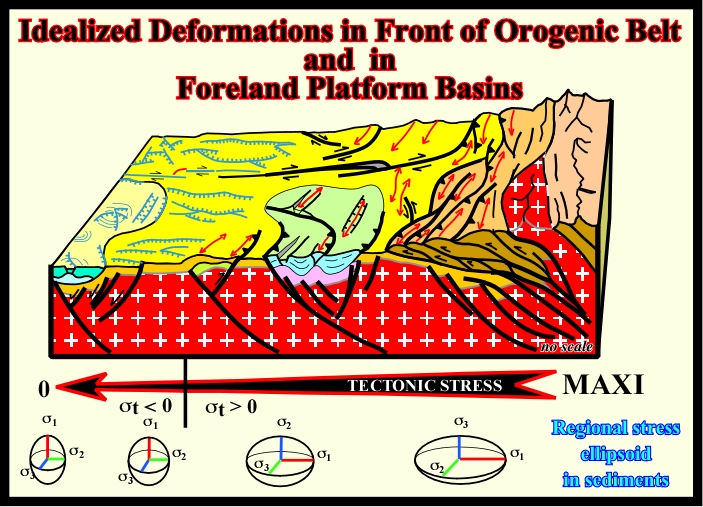
Fig. 14- This sketch illustrates the conjecture that the tectonic stress decrease, progressively, in direction of the craton, that is to say, away from the orogenic belt. Actually, the tectonic stress is more or less constant within the considered lithospheric plate. However, as the strength to deformation of the rocks change, deformation occurs where the sediments cannot stand anymore the effective stresses. In such a tectonic setting, when σ1 is vertical, salt layers, if they were deposited will be deformed in salt ridges striking perpendicularly to the cylindrical-folds and thrusts of the fold-belt.
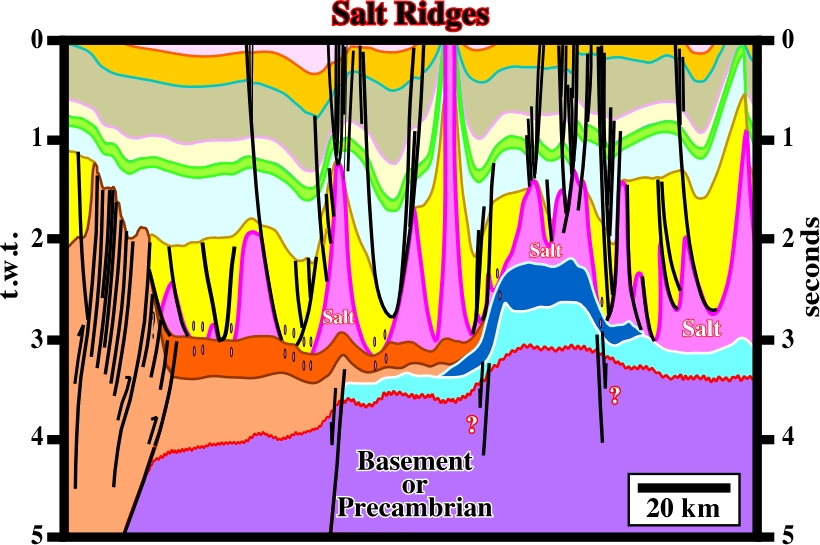
Fig. 15- In the Caspian Sea, nearby the huge Kasaghan oil discovery (dark blue), salt ridges strike perpendicularly to the thrust-faults and cylindrical-folds of the fold-belt (in the left end of this tentative geological interpretation of a seismic line). Therefore, is quite possible than they were created by the lessening tectonic regime (see Tables I and II). The majority of the salt ridges were formed before the unconformity at the top of the yellow interval. However, some of them were reactivate, later, by another tectonic regime, in which halokinesis seems quite active with formation of diapirs.
1.4.4- Equilibrium (Halokinesis), σt = 0 (see Table II)
This tectonic regime occurs when the tectonic stress is nil (σt = 0). It is an extensional tectonic regime characterized by a vertically oblong biaxial effective stresses ellipsoid: σ1 is vertical and σ2 and σ3are horizontal and equals. In such a tectonic setting, when a salt layer is present, due to the salt properties (see later), it can be deformed by lateral or vertical flowage (a progressive change in shape occurring without breaking), creating local compensatory subsidence, which will control the accommodation of the syn-kinematic sediments.
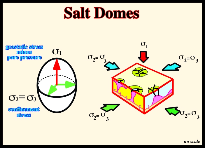
Fig. 16- As illustrated in the block diagram, the faulting associated with this tectonic regime is characterized by normal faults striking in all directions (σ2= σ3). This fault pattern is also, often, recognized on antiform structures created by differential compaction. When, a thick mobile layer (salt or under-compacted shales) is present, even in absence of a significant tectonic stress, it can flow by itself. Halokinesis designates the salt and overburden deformations taking place in such a tectonic setting (absence of a tectonic stress), while argilokinesis denotes the deformations associated with an under-compacted shale interval.
Under such tectonic conditions, the normal-faults lengthening the sediments (overburden, when a salt layer is present) strike in all azimuths (“radial faults”). Theoretically, radial normal-faults are created in order to solve a volume problem. When a salt layer flows upward, due to the contrast of density between the salt and the surrounding sediments, it creates a more or less circular salt diapir and thereby the overburden is lengthened around it. As lengthening creates a potential void and as nature dislikes vacuity, radial normal-faults extend the overburden in order to fill the space created. Theoretically, in a cross-section, the addition of the opposite normal fault throws should be roughly zero. Admittedly, halokinesis is not limited to a homogeneous upward flowage of salt. As we see later, from physics standpoint, salt diapirs, with vertical walls, are stable structures. The salt of the upper part of salt diapirs is forced to flow laterally, since contrariwise to sediments, the density of salt rock does not change with depth (salt cannot be compacted). The density of the surrounding sediments increases with depth due to compaction.
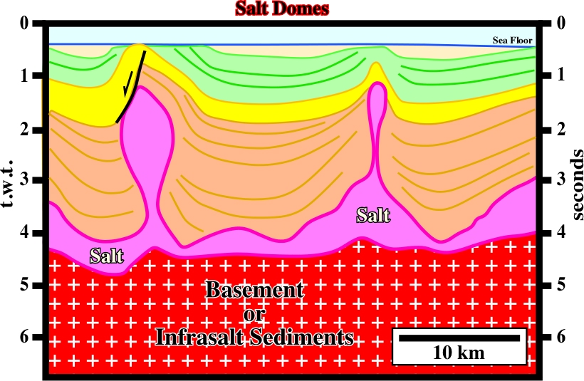
Fig. 17- In Nordkap basin (Barents Sea), the basement is not involved in deformation (at least in the area where the seismic line of this tentative geological interpretation was shot). The salt induced tectonic disharmony at the bottom of the salt separates the infra-salt strata (basement and infra-salt strata) from the cover (salt + overburden). The small undulations at the bottom are seismic pitfalls induced by salt thickness lateral changes. In absence of significant tectonic stress, the thick Permian salt layer flowed upward forming quite large salt diapirs, which deformed the overburden. Notice that flanks of the diapiric structures are not vertical (physical impossibility) and the overburden, seems to be, mainly, pre-kinematic (regionally, the overburden shows a northward thickening).
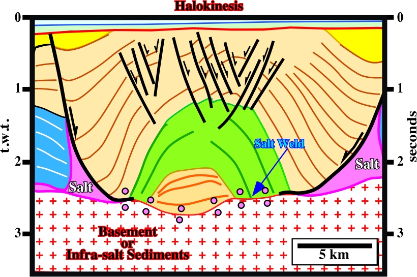
Fig. 18- This antiform structure is a typical extensional structure created by halokinesis. The lateral depocenters are syn-kinematic intervals deposited in association with a compensatory subsidence created by salt flowage. The core of the structure, which is, mainly, pre-kinematic, was inverted by halokinesis. The reflectors of the pre-kinematic intervals (brown and green) have a, more or less, convergent internal configuration, while those of the syn-kinematic interval have a divergent internal configuration toward the fault welds (surface or zone joining strata or originally separated by autochthonous or allochthonous salt, equivalent to a salt weld along which there has been significant slip or shear). The normal-faults (with opposite vergence) near the apex of the structure, strongly, extend the overburden. The salt induced tectonic disharmony, between the infra-salt strata and the cover (salt + overburden, is underlined by the bottom of the salt and an associated salt weld.
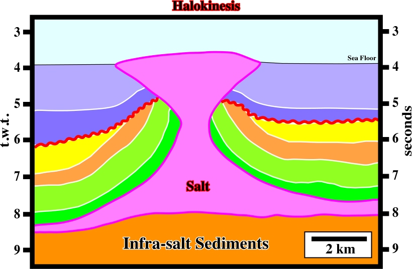
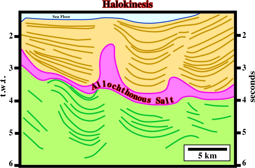
Fig. 20- Halokinesis can create complex structures particularly when there is superimposition of autochthonous and allochthonous salt structures, as is the case on this seismic line from Garden Banks (deep-water Gulf of Mexico), where two salt-induced tectonic disharmonies can predicted. When a significant sat weld is formed in the allochthonous salt the salt tectonic disharmony becomes a décollement surface. The salt weld joining strata originally separated by gently dipping allochthonous salt sheets is a tertiary salt weld (see later).
1.4.5- Rifts – Extensional Strike-Slip, σ1 < 0 (see Table II)
Under this tectonic regime, which is characterized by a vertically oblong triaxial effective stresses ellipsoid with σ1 vertical, and σ2 and σ3horizontal, the cover (salt + overburden) is lengthened, whether the basement is involved or not in the deformation. When a salt layer is present, it can be deformed in salt ridges (fig. 21) or in growth-faults (fig. 22).
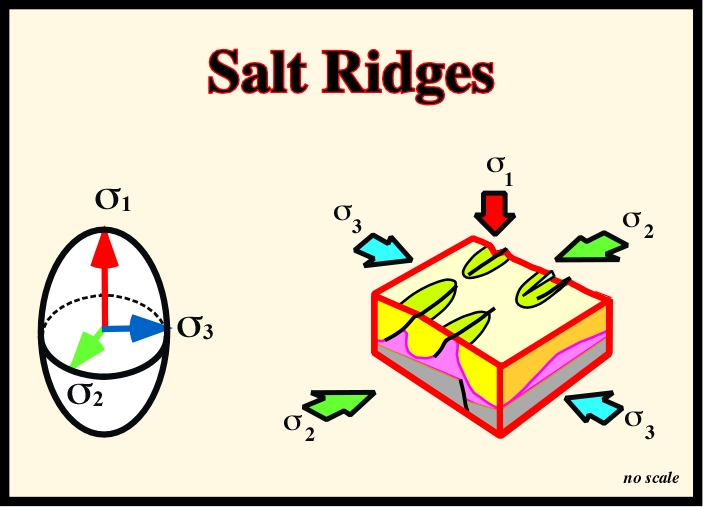
Fig. 21- Salt ridges are parallel to σ2. They form extensional structures in the overburden. In Atlantic-type divergent margin, where this tectonic regime is common, salt ridges are, generally, parallel to the shoreline (fig.23). When the salt induced tectonic disharmony is slightly tilted seaward. asymmetric syn-kinematic depocenters are formed in the overburden. Salt ridges can be are rooted with faults or fracture zones of the infra-salt strata.
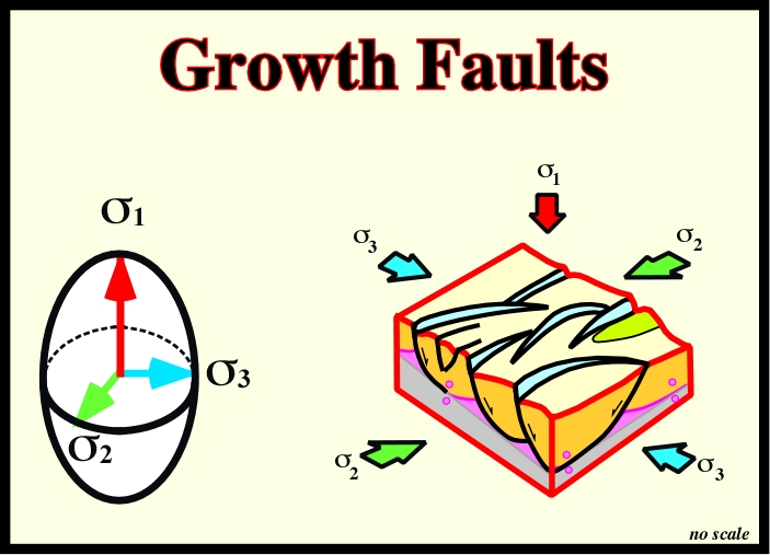
Fig. 22- A growth fault is a syn-sedimentary normal fault with thicker strata in the hanging-wall. Generally, in a growth fault, two sections can be recognized: a) The pre-growth or pre-kinematic section and b) The growth section, which exhibits both contemporaneous movement and post-depositional movement on all beds but the upper one. The displacement of a growth fault expands a stratigraphic unit, so the hanging-wall is thicker than the foot-wall. The movement of the fault creates more "room" (accommodation or space available for sedimentation) for deposition in down-thrown side. Growth faults are common in Atlantic and non Atlantic-type divergent margins, in which a salt interval or a mobile shale layers were deposited. As depicted the growth faults are curvilinear but rarely listric, in spite of the fact that they flatten and die, in depth, against a mobile layer (salt or shales). Similarly, relay structures, i.e., zones connecting the foot-walls and hanging-walls of overlapping fault segments, and relay ramps (the transfer of displacement) are quite frequent in association with growth faults
Very often, growth-faults are associated with salt ridges. Therefore, generally, it is difficult to differentiate a salt ridge with a growth-fault, from a simple growth-fault developed on a mobile salt substratum. The best criterion, as pictured on the previous block diagrams, seems to be the cartographic geometry:
(i) Salt ridges have a more or less unbent geometry. The normal-faults associated with them are more or less rectilinear.
(ii) Growth-faults have a curvilinear geometry. Therefore, individually, they create a non-homogeneous extension. So, the association of an indefinite number of growth-faults is required (curvilinear-faults are often called listric faults because in a cross-section, they have a decreasing hade). The term listric comes from the Greek « listron », which means shovel, what is not synonym of decreasing hade. Up-dip, a listric fault has a normal geometry, while down-dip, its geometry becomes reverse).
At the ground surface and on time contour maps, very often, the cartography of the growth faults is in relay. The maximum extension (maximum throw) of one fault is relayed with the minimum of extension (minimum throw) of the next fault (see fig. 23). Such geometry allows homogeneous lengthening (without wrenching). On this subject, it is important to remember that all curvilinear faults (normal or reverse) have a maximum extension (maximum throw) between the ends, where the extension is zero.
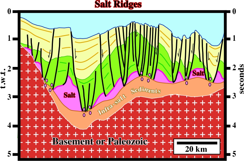
Fig. 23- The lengthening of the sediments is evident. The tectonic regime is characterized by σ1 vertical. The antiform morphology of the sea bottom is quite significant. The majority of the normal-faults die on the tectonic disharmony associated with the salt layer (bottom of the salt). The sediments above and below the tectonic disharmony show different deformations. Above it, the cover, that is to say, the salt and overburden have been, strongly, extended (the extension still is going on). Below the tectonic disharmony, the infra-salt strata are just, slightly, deformed. The cartography of the salt structures, which are bordered by normal-faults, indicates they have a more or less rectilinear geometry. Thereby, they can be classified as salt ridges striking parallel to σ2.
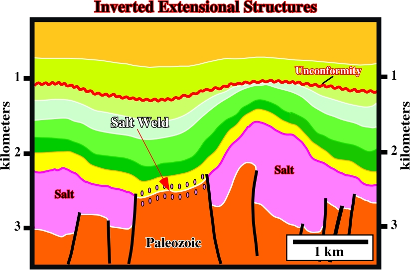
Fig. 24- The salt weld in the central part of the line suggests that before deformation the salt layer was continuous between the yellow and brown interval. Then, the infra-salt strata (Paleozoic) were lengthened by normal-faults creating potential voids that were filled by salt (“salt grabens”) due to a lateral salt flowage, which created a window in the salt layer. Later, a compressional tectonic regime shortened the area inverting the salt grabens. All sedimentary column was uplifted creating a significant relative sea level fall which induce an important erosional surface (red unconformity). A new marine ingression allowed the deposition of the post-unconformity intervals. However, taken into account the morphology of the unconformity, a slightly reactivation of the compressional tectonic regime cannot be excluded, even if it can be explained as the result of a differential compaction.
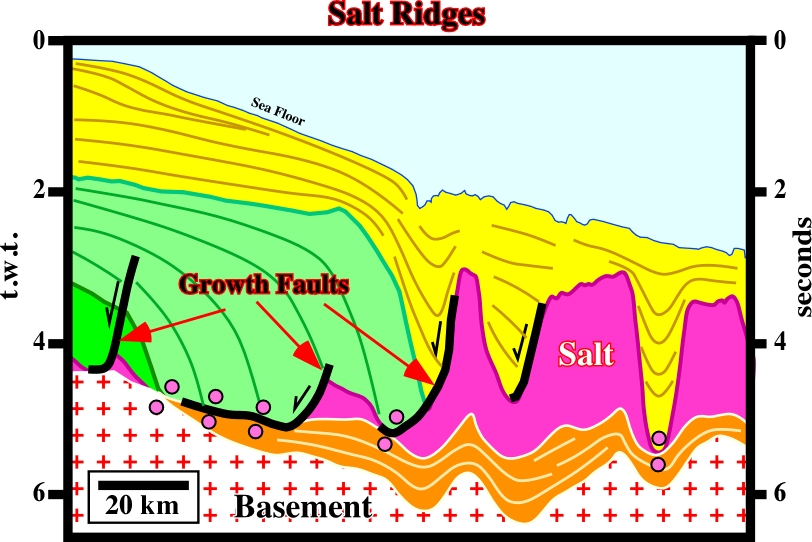
Fig. 25- Salt ridges and growth faults are frequent in Santos geographic basin (Brazil offshore). Taking into account that the deformation of the infra-salt strata is apparent and due to velocity-changes induced lateral thickness changes of the salt layer, which creates pull-ups and pull-down, one can say that below the tectonic disharmony the sediments are almost undeformed. Above it, that is to say, in the cover (salt + overburden) salt ridges and growth faults extended the overburden. Notice, the dip of the salt induced tectonic disharmony is in time. In a depth converted data, which is closer to the reality, the dip is ,clearly, landward (to the left). In fact, on a seismic line (time profile), the progressive seaward increasing in water depth, delay the seismic waves. The seismic reflectors are, gradually, pulled-down as the water depth increases.
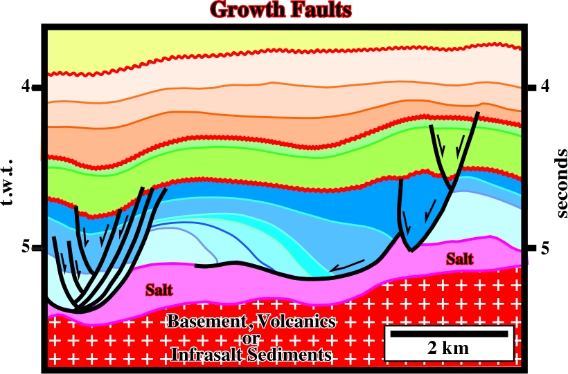
Fig. 26- In Angola deep water, Cretaceous sediments and particularly the Pinda formation (carbonate facies), which is a potential reservoir interval in the shelf, were extended by growth-faults developed on the top of the salt layer due to an extensional tectonic regime characterized by σ1 vertical, σ2 horizontal striking more or less N-S and σ3 horizontal and W-E. The accommodation (space available for sediments) developed in the hanging-wall of the growth faults is, partially, due to the salt flowage, which creates a compensatory subsidence and, partially, due an onset of raft tectonics (extreme extension characterized by the opening of deep, syn-sedimentary grabens and separation of intervening overburden into rafts , which slide down-slope on a décollement of thin salt, like a block-glide landslip)
1.5- Summary of Salt Extensional Tectonic Deformation (see Table III)
Before reviewing the basic principles of halokinesis, on table III, we will sum up the main extensional deformations associated with a mobile salt layer. The tridimensional geometry of the structures:
(i) Salt Ridges (σt> 0)
(ii) Halokinetic Structures (σt= 0)
(iii) Salt Ridges, Growth Faults, Gravity Sliding (σt < 0)
and the associated time contour maps are proposed. Special attention should be paid to the proposed block diagrams in order to better understand the second part of this short course, in which 3D seismic data is used. Indeed, it is important to realize that a time slice is just a geological map with a flat topography. However, time-slices, as well as geological maps without topography, are not necessary similar to time contour maps. This is particularly true for the geometry of the fault planes. In fact, as shown by G. Dickinson (1954), the effects of intersecting faults in sub-surface and time contours maps are very difficult to comprehend, especially, in no flat geological maps due to topography effect. Ex: In a time contour map, when two normal faults affecting horizontal strata intersect, it is the younger fault that is displaced and not the older one.
Table III
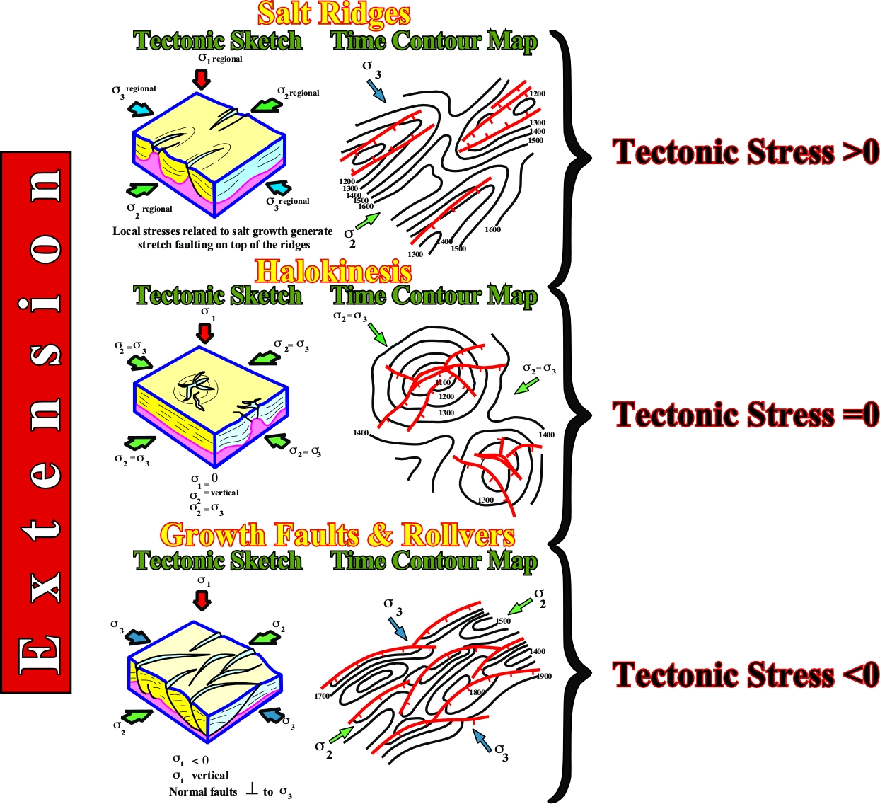
It is interesting to notice that long graben structure in the overburden are typically associated with salt ridges (σt > 0), radial normal faults to diapirs (σt= 0) and relay structures and relay ramps relay ramps (transfer of displacement) to growth faults (σt< 0).
to continue press
next
![]()